Mechanistic disease models are at the heart of disease ecology and have generated fundamental biological insights, ranging from our understanding of disease-density thresholds to the influence of host heterogeneity on the spread of disease. The definition of a mechanistic model is actually debated quite a lot, but here I am referring specifically to systems of ordinary differential equations (ODEs) that can capture the important non-linearities and temporal dynamics of infection, which are founded on the idea of transmission from infectious hosts to susceptible hosts. This is probably the simplest example:
\[\begin{align} \frac{dS}{dt} & = - \beta S I \\ \frac{dI}{dt} & = \beta S I - \gamma I \\ \frac{dR}{dt} & = \gamma I \end{align}\]In this simple $SIR$ model, $S$, $I$, and $R$ represent the fraction of susceptible, infected, and removed hosts, respectively, where $S + I + R = 1$. $\beta$ represents the frequency-dependent transmission, where $\beta S I$ informs the rate at which new individuals become infected, as a proportion of the total population. And, finally, $\gamma$ is the rate of death due to infection (i.e. virulence). In some models this is considered the recovery or immune rate. I’m assuming, among other things, that there is no recovery, only death due to infection.
Because mechanistic models like this one do such a good job at capturing the non-linear dynamics of infection, they are often used as predictive tools to inform, for instance, how vaccination or climate change or (insert your favorite meme) might influence disease epidemics. However, it is rare to see these models parameterized in rigorous ways, likely because this can involve complicated experiments that might be infeasible, say, in human systems. Moreover, non-linear model-fitting routines can be computationally costly and might lie outside the expertise of field ecologists who collect the necessary data.
However, if we collect our data in simple, yet calculated, ways, new technologies make model-fitting a surmountable challenge. And model-fitting can help get us those coveted parameter estimates that we need to make predictions. Furthermore, if model-fitting is done in a Bayesian framework, in cases where some parameters can be estimated with experimental data, we can combine information from the lab and from the field in a rigorous analysis. For instance, we can fit a mechanistic model to epidemic data collected from the field, and we can use experimental measurements of some or all model parameters to construct prior likelihoods.
In this blog post, I will show how we can fit a simple, mechanistic $SIR$ model to simulated data - representing easily collected data from the field - using R and Stan.
First, I will generate data by integrating an $SIR$ model with known $\beta$ and $\gamma$ parameters. This will simulate an epidemic window, which represents a time period over which data can be collected. For instance, we can go to the field and measure the proportion of hosts infected at various time points to capture the rise and fall of infection. This data is used to fit the model.
# Load some required packages
##############
library(deSolve)
library(dplyr)
library(ggplot2)
library(rstan)
rstan_options(auto_write = TRUE)
options(mc.cores = parallel::detectCores())
##############

# To simulate the data, we need to assign initial conditions.
# In practice, these will likely be unknown, but can be estimated from the data.

I0 = 0.02    # initial fraction infected
S0 = 1 - I0 # initial fraction susceptible
R0 = 0

# Assign transmission and pathogen-induced death rates:
beta = 0.60
gamma = 0.10

# We will use the package deSolve to integrate, which requires certain data structures.
# Store parameters and initial values
# Parameters must be stored in a named list.
params <- list(beta = beta,
              gamma = gamma)

# Initial conditions are stored in a vector
inits <- c(S0, I0, R0)

# Create a time series over which to integrate.
# Here we have an epidemic that is observed over t_max number of days (or weeks or etc).
t_min = 0
t_max = 50
times = t_min:t_max

# We must create a function for the system of ODEs.
# See the 'ode' function documentation for further insights.
SIR <- function(t, y, params) {
  with(as.list(c(params, y)), {

    dS = - beta * y[1] * y[2]

    dI = beta * y[1] * y[2] - gamma * y[2]

    dR = gamma * y[2]

    res <- c(dS,dI,dR)
    list(res)
  })
}

# Run the integration:
out <- ode(inits, times, SIR, params, method="ode45")

# Store the output in a data frame:
out <- data.frame(out)
colnames(out) <- c("time", "S", "I", "R")

# quick plot of the epidemic
plot(NA,NA, xlim = c(t_min, t_max), ylim=c(0, 1), xlab = "Time", ylab="Fraction of Host Population")
lines(out$S ~ out$time, col="black")
lines(out$I ~ out$time, col="red")
legend(x = 30, y = 0.8, legend = c("Susceptible", "Infected"),
       col = c("black", "red"), lty = c(1, 1), bty="n")
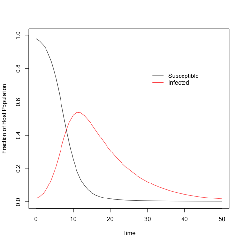
The parameters represent a particularly virulent pathogen, where by the end of 50 days, most of the population has been infected and has died. This gives us the “true” epidemic dynamics of the system, from which we can simulate data that an ecologist might collect. For instance, an ecologist could go to the field and sample a given number of individuals from the population and figure out how many are infected. This could be repeated a number of times throughout the epidemic period, as follows:
sample_days = 20 # number of days sampled throughout the epidemic
sample_n = 25 # number of host individuals sampled per day

# Choose which days the samples were taken.
# Ideally this would be daily, but we all know that is difficult.
sample_time = sort(sample(1:t_max, sample_days, replace=F))

# Extract the "true" fraction of the population that is infected on each of the sampled days:
sample_propinf = out[out$time %in% sample_time, 3]

# Generate binomially distributed data.
# So, on each day we sample a given number of people (sample_n), and measure how many are infected.
# We expect binomially distributed error in this estimate, hence the random number generation.
sample_y = rbinom(sample_days, sample_n, sample_propinf)
Now that we have some synthetic data, let’s fit the mechanistic model using the Stan MCMC sampling software. I would highly recommend consulting the Stan documentation for fitting ODEs, but I’ll do my best to annotate the model statement. In the model, we’ll estimate the two parameters of interest $\beta$ and $\gamma$, as well as the initial conditions, which were likely unknown in the field.
# The Stan model statement:
cat(
'
functions {

  // This largely follows the deSolve package, but also includes the x_r and x_i variables.
  // These variables are used in the background.

  real[] SI(real t,
            real[] y,
            real[] params,
            real[] x_r,
            int[] x_i) {

      real dydt[3];

      dydt[1] = - params[1] * y[1] * y[2];
      dydt[2] = params[1] * y[1] * y[2] - params[2] * y[2];
      dydt[3] = params[2] * y[2];

      return dydt;
    }

}

data {
  int<lower = 1> n_obs; // Number of days sampled
  int<lower = 1> n_params; // Number of model parameters
  int<lower = 1> n_difeq; // Number of differential equations in the system
  int<lower = 1> n_sample; // Number of hosts sampled at each time point.
  int<lower = 1> n_fake; // This is to generate "predicted"/"unsampled" data

  int y[n_obs]; // The binomially distributed data
  real t0; // Initial time point (zero)
  real ts[n_obs]; // Time points that were sampled

  real fake_ts[n_fake]; // Time points for "predicted"/"unsampled" data
}

transformed data {
  real x_r[0];
  int x_i[0];
}

parameters {
  real<lower = 0> params[n_params]; // Model parameters
  real<lower = 0, upper = 1> S0; // Initial fraction of hosts susceptible
}

transformed parameters{
  real y_hat[n_obs, n_difeq]; // Output from the ODE solver
  real y0[n_difeq]; // Initial conditions for both S and I

  y0[1] = S0;
  y0[2] = 1 - S0;
  y0[3] = 0;

  y_hat = integrate_ode_rk45(SI, y0, t0, ts, params, x_r, x_i);

}

model {
  params ~ normal(0, 2); //constrained to be positive
  S0 ~ normal(0.5, 0.5); //constrained to be 0-1.

  y ~ binomial(n_sample, y_hat[, 2]); //y_hat[,2] are the fractions infected from the ODE solver

}

generated quantities {
  // Generate predicted data over the whole time series:
  real fake_I[n_fake, n_difeq];

  fake_I = integrate_ode_rk45(SI, y0, t0, fake_ts, params, x_r, x_i);

}

',
file = "SI_fit.stan", sep="", fill=T)

# FITTING

# For stan model we need the following variables:

stan_d = list(n_obs = sample_days,
              n_params = length(params),
              n_difeq = length(inits),
              n_sample = sample_n,
              n_fake = length(1:t_max),
              y = sample_y,
              t0 = 0,
              ts = sample_time,
              fake_ts = c(1:t_max))

# Which parameters to monitor in the model:
params_monitor = c("y_hat", "y0", "params", "fake_I")

# Test / debug the model:
test = stan("SI_fit.stan",
            data = stan_d,
            pars = params_monitor,
            chains = 1, iter = 10)

# Fit and sample from the posterior
mod = stan(fit = test,
           data = stan_d,
           pars = params_monitor,
           chains = 3,
           warmup = 500,
           iter = 1500)

# You should do some MCMC diagnostics, including:
#traceplot(mod, pars="lp__")
#traceplot(mod, pars=c("params", "y0"))
#summary(mod)$summary[,"Rhat"]

# These all check out for my model, so I'll move on.

# Extract the posterior samples to a structured list:
posts <- extract(mod)
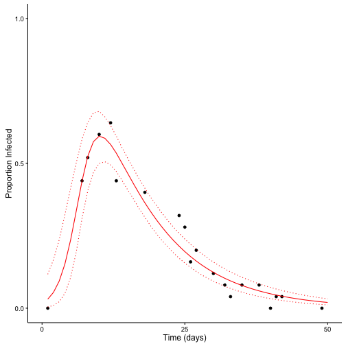
Now we can validate the model. We’ll see how well our the Stan model fits to the synthetic data and we adequately estimate the known parameter values.
# Check median estimates of parameters and initial conditions:
apply(posts$params, 2, median)
## [1] 0.6865799 0.0926325apply(posts$y0, 2, median)[1:2]## [1] 0.98243659 0.01756341# These should match well.
#################
# Plot model fit:
# Proportion infected from the synthetic data:
sample_prop = sample_y / sample_n
# Model predictions across the sampling time period.
# These were generated with the "fake" data and time series.
mod_median = apply(posts$fake_I[,,2], 2, median)
mod_low = apply(posts$fake_I[,,2], 2, quantile, probs=c(0.025))
mod_high = apply(posts$fake_I[,,2], 2, quantile, probs=c(0.975))
mod_time = stan_d$fake_ts
# Combine into two data frames for plotting
df_sample = data.frame(sample_prop, sample_time)
df_fit = data.frame(mod_median, mod_low, mod_high, mod_time)
# Plot the synthetic data with the model predictions
# Median and 95% Credible Interval
ggplot(df_sample, aes(x=sample_time, y=sample_prop)) +
geom_point(col="black", shape = 19, size = 1.5) +
# Error in integration:
geom_line(data = df_fit, aes(x=mod_time, y=mod_median), color = "red") +
geom_line(data = df_fit, aes(x=mod_time, y=mod_high), color = "red", linetype=3) +
geom_line(data = df_fit, aes(x=mod_time, y=mod_low), color = "red", linetype=3) +
# Aesthetics
labs(x = "Time (days)", y = "Proportion Infected") +
scale_x_continuous(limits=c(0, 50), breaks=c(0,25,50)) +
scale_y_continuous(limits=c(0,1), breaks=c(0,.5,1)) +
theme_classic() +
theme(axis.line.x = element_line(color="black"),
axis.line.y = element_line(color="black"))
The Stan model does a good job estimating the parameters and predicting unobserved data.
Admittedly, this “simple” approach will not work in some cases. For example, I cannot think of a good way to fit systems of stochastic differential equations in Stan, where the likelihood has to be averaged across many realizations of the system. Or, for models that have to estimate the number of, say, exposed or infected classes, which is an integer. Stan does not allow integer parameters, at least not yet. In my postdoc I am using custom MCMC scripts in C, which allows for fast integration with Monte MISER. This is certainly more challenging, though.

Leave a Comment