
This blog has a few goals. First, you’ll see how to simulate a nested data set using the assumptions of a linear mixed-effects model. Then, you’ll learn about R packages that can help to summarize and visualize similar hierarchical data in fast, reproducible, and easily generlizable ways. Finally, the user can change the simulation parameters to visualize the emergent effects of variability at different hierarchical scales.
Data Generation
Working with hierarchical data can be a pain, but there is a suite of R packages in the tidy family that are unbelievably helpful. What I mean is that these packages will change your scientific life forever. For real.
Hyperbole aside, let’s start by generating some realistic, nested data. We’ll be testing Bergmann’s rule that body size increases with elevation (as a proxy for temperature) by sampling along different mountains. We’ll sample multiple individuals of many species, representing many genera, sampled across multiple mountains. Lots of nestedness here.
There’s a lot of non-independence going on with this type of nested sampling. You’d expect body size to vary more among genera than among species within a given genera, and there is probably variation among mountains. This all affects the intercept of body size (i.e. the average body size within groups). There might be similar non-independence in the relationship between body size and elevation (i.e. the slope). We’ll code this type of non-independence as random effects on the interecept and slope, below.
This blog is focused on managing and visualizing hierarchical data. In a later post, I’ll use a very similar generative example to illustrate proper statistical models to handle all of this non-independence.
## Sample sizes:
mount_N <- 10 # Number of mountains sampled
obs_N_perMount <- sample(c(100:300), size=mount_N, replace=T)
obs_N <- sum(obs_N_perMount)
# Note: the same species could be found on different mountains
genera_N <- 15 # Number of genera
species_N_perGenus <- sample(c(2:8), size=genera_N, replace=T) # Number of species per genus
species_N <- sum(species_N_perGenus)

## Create placeholders
# Make sure these are factors, which will be used later.
Mount <- factor(rep(c(1:mount_N), times=obs_N_perMount))
Genera <- factor(sample(c(1:genera_N), size=obs_N, replace=T))
Species <- factor(sample(c(1:species_N), size=obs_N, replace=T))

## Now assign parameters that determine the relationship between elevation and body size
beta_mean <- 2.0 # Slope: Body size increases with elevation
alpha_mean <- 0.0 # Intercept: Mean body size (centered)

# Random effects on slope
species_sd_beta <- 0.5
genera_sd_beta <- 2.5
mount_sd_beta <- 1.0

species_rand_beta <- rnorm(species_N, 0, species_sd_beta)
genera_rand_beta <- rnorm(genera_N, 0, genera_sd_beta)
mount_rand_beta <- rnorm(mount_N, 0, mount_sd_beta)

# Random effects on intercept
species_sd_alpha <- 2.5
genera_sd_alpha <- 10.0
mount_sd_alpha <- 2.5

species_rand_alpha <- rnorm(species_N, 0, species_sd_alpha)
genera_rand_alpha <- rnorm(genera_N, 0, genera_sd_alpha)
mount_rand_alpha <- rnorm(mount_N, 0, mount_sd_alpha)

## Elevation (centered and scaled)
Elevation <- rnorm(obs_N, 0, 1)

## Generate body weights
# Note: Because we generated the data above in a smart way, we can vectorize this process!
Weight <- vector(mode="numeric", length=obs_N)
# Add the intercept with random effects:
Weight <- alpha_mean + species_rand_alpha[Species] + genera_rand_alpha[Genera] + mount_rand_alpha[Mount]
# Add the slope with random effects:
Weight <- Weight +
          (beta_mean + species_rand_beta[Species] + genera_rand_beta[Genera] + mount_rand_beta[Mount]) * Elevation

# Put this into a data frame:
berg <- data.frame(Mount, Genera, Species, Elevation, Weight)
head(berg)
## Mount Genera Species Elevation Weight
## 1 1 2 13 -0.11214172 18.419632
## 2 1 8 50 0.84987820 7.974134
## 3 1 7 63 -1.84140031 12.169132
## 4 1 13 24 -0.06470968 18.033449
## 5 1 6 47 -3.26612214 -4.809293
## 6 1 4 40 -0.75520574 5.805547Very crudely, let’s look at the overall pattern in the data.
plot(berg$Weight ~ berg$Elevation, pch=20, xlab="Elevation", ylab="Weight")
Well, that’s a lot of variation, which makes it hard to see a clear pattern. Does the inherent hierarchy in the data obscure the body size - elevation relationship? What are the patterns among mountains? Among genera? Among species?
Data Management and Synthesis
I’m going to focus on the tidy family of packages that can helpu us dissect and summarize the raw data in simple and reproducible ways, and we’ll use the ggplot2 package for visualization.
# Launch all of the 'tidy' packages.
library(tidyverse)
## Loading tidyverse: ggplot2
## Loading tidyverse: tibble
## Loading tidyverse: tidyr
## Loading tidyverse: readr
## Loading tidyverse: purrr
## Loading tidyverse: dplyrBrad Boehmke does a great job of highlighting the functions of the dplyr and tidyr packages in his R publication, and you should definitely read it. I’ll just highlight a few useful functions relevant to this dataset.
Here’s a simple question: What are the average body weights and their standard deviations on each mountain? We could write a for-loop that partitions the data frame and then calculates and stores these summary statistics, but that is pretty inefficient and prone to errors. Instead, use dplyr and the summarize() function.
# The '%>%' symbol pipes the object on the left to the function on the right
# 'group_by() clusters all of the data for the given variables
# 'summarize()' creates new columns and applies functions to available variables

berg %>%
  group_by(Mount) %>%
  summarize(Weight_avg = mean(Weight), Weight_sd = sd(Weight))
## # A tibble: 10 × 3
## Mount Weight_avg Weight_sd
## <fctr> <dbl> <dbl>
## 1 1 2.75987283 8.980855
## 2 2 1.84340717 8.879757
## 3 3 0.34929020 9.655934
## 4 4 -3.99058099 9.603364
## 5 5 1.04847069 8.622723
## 6 6 3.36407484 8.667651
## 7 7 -2.16678716 9.902605
## 8 8 0.03388973 8.597225
## 9 9 -1.21115250 8.011652
## 10 10 0.25712038 8.938851What about the mean weights of genera on different mountains?
# Now cluster by Mount and Genera
# print() can be used to specify how many columns to print to screen

berg %>%
  group_by(Mount, Genera) %>%
  summarize(Weight_avg = mean(Weight), Weight_sd = sd(Weight)) %>%
  print(n=20)
## Source: local data frame [150 x 4]
## Groups: Mount [?]
##
## Mount Genera Weight_avg Weight_sd
## <fctr> <fctr> <dbl> <dbl>
## 1 1 1 -4.4544981 3.557380
## 2 1 2 18.5225092 2.642183
## 3 1 3 3.5370207 3.253391
## 4 1 4 1.7430990 2.816731
## 5 1 5 -9.2871199 3.045857
## 6 1 6 6.7972462 4.148961
## 7 1 7 13.2109473 3.133184
## 8 1 8 4.2826290 3.119941
## 9 1 9 -1.9444854 2.278156
## 10 1 10 3.3850735 3.412358
## 11 1 11 0.2992717 1.924521
## 12 1 12 -13.4347891 4.312500
## 13 1 13 15.4608036 2.652208
## 14 1 14 7.5510452 3.584307
## 15 1 15 13.9542854 3.228134
## 16 2 1 -6.2408338 3.316820
## 17 2 2 15.6266652 2.730077
## 18 2 3 3.4377517 3.139546
## 19 2 4 -0.7654253 3.229899
## 20 2 5 -12.2088844 3.346544
## # ... with 130 more rowsPerhaps simpler, we want to know how many species were found on each mountain.
berg %>%
  group_by(Mount) %>%
  summarize(species_N_perMount = length(unique(Species)))
## # A tibble: 10 × 2
## Mount species_N_perMount
## <fctr> <int>
## 1 1 65
## 2 2 62
## 3 3 55
## 4 4 66
## 5 5 57
## 6 6 64
## 7 7 60
## 8 8 65
## 9 9 63
## 10 10 66Data Visualization
We can even pipe these data frames right into ggplot2! Let’s take a look at the variability in average weights across the different mountains. Here we’ll average to the species level, because we have multiple individuals sampled from each species, and we’ll summarize these species-level averages using boxplots.
# Cluster by Mount and Species
# Pipe to ggplot(), and the data frame argument will be implied

berg %>%
  group_by(Mount, Species) %>%
  summarize(Weight_avg = mean(Weight)) %>%
  ggplot(aes(y=Weight_avg, x=Mount)) +
  geom_boxplot()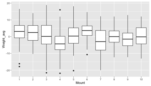
Now, more relevant to the question at hand, what is the relationship between body size and elevation? First, is it consistent across mountains? Let’s look at this visually. We’ll use the facet_wrap() function from the ggplot2 package.
ggplot(berg, aes(x=Elevation, y=Weight))+
  geom_point(shape=20)+
  facet_wrap(~Mount, ncol=5)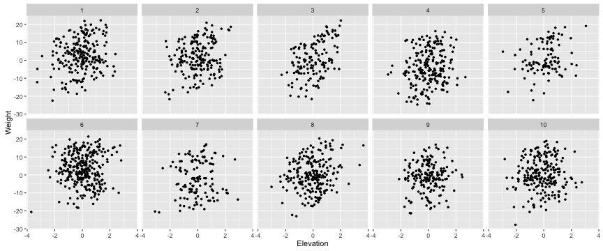
It would appear that Bergmann’s rule does not apply to these mountains. What’s going on?
Let’s use facet_wrap() to look at the each genus separately, and let’s highlight the species with different colors.
# We'll suppress the Species legend, because we have so many species 'guides(color=F)'

ggplot(berg, aes(x=Elevation, y=Weight, color=Species))+
  geom_point(shape=20)+
  facet_wrap(~Genera, ncol=5)+
  guides(color=F)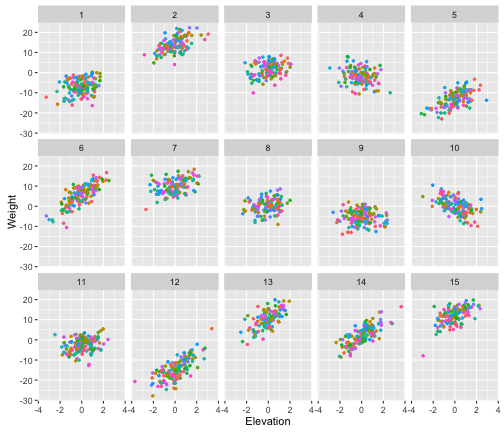
Now it becomes clear why Bergmann’s rule was being obscured when we looked across the whole data set and when we looked at mountains individually. There is a lot of variation among genera in the body size - elevation relationship. This makes sense, because we coded a large random variation in slope among genera.
Go back and change the random variation in slopes and intercepts at the different hierarchical levels. How does this affect the overall pattern among mountains? This type of simulation can help you understand how much data you might need to collect in order to find statistically meaningful patterns.
Leave a Comment